By Cristina Lincaru, Adriana Grigorescu and Speranța Pîrciog, INCSMPS – National Scientific Research Institute for Labour and Social Protection, Bucharest, Romania. Corresponding author: cristina.lincaru@incsmps.ro

Intersectoral reallocation—the changing distribution of employment across activities—is a central mechanism of structural transformation, but its regional geography within the knowledge economy remains uneven. This study uses annual changes in NUTS 2 employment shares as aggregate regional signals of intersectoral mobility across five overlapping Eurostat dimensions: HTC, KIS, KIS_HTC, NACE J and NACE M. A sector-specific Structural Change Intensity (SCI) is mapped through five Space–Time Cubes and Emerging Hot Spot Analysis for 2009–2025. Because the data do not track individual workers, mobility is interpreted as structural reweighting rather than observed worker flows. High–SCI clustering is sparse and geographically selective: HTC and KIS_HTC each show three consecutive hot spots; J shows four new and three sporadic hot spots; KIS shows one new and three sporadic; and M shows one consecutive and two sporadic. Most detected trajectories lie in a northern-to-northwestern/central European arc, with isolated southern outliers. The findings frame regional adaptation as an uneven geography of structural reallocation rather than a uniform knowledge-economy transition.

Introduction

Structural transformation is fundamentally a process of reallocating economic activity across sectors (Herrendorf et al., 2014). For regional labour markets, this matters because sectoral reweighting changes where jobs and skill demands are created or displaced. Regional adaptation is therefore not only the capacity to sustain employment, but the ability to accommodate structural change and develop new growth paths (Boschma, 2015). Recent OECD evidence likewise shows that structural shocks produce substantial reallocation across industries in exposed places, while actual worker mobility between industries can remain limited (OECD, 2026).

In this paper, intersectoral mobility is used in a structural, not micro-flow, sense. The data do not identify workers moving from one sector to another; instead, year-to-year changes in each activity’s share of regional employment reveal where the internal sectoral composition is being reweighted. The questions are where this reallocation is intense, whether it forms spatial-temporal clusters, and what those clusters imply for uneven regional adaptation in Europe’s knowledge economy. Because the selected Eurostat indicators overlap, the analysis compares their trajectories rather than summing them into a single mobility index.

Data

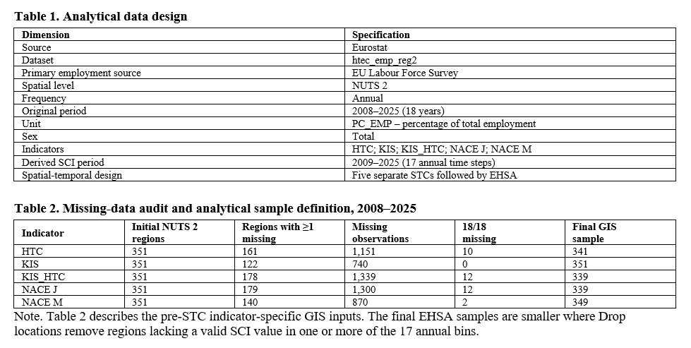
The analysis uses annual NUTS 2 employment shares from Eurostat’s htec_emp_reg2 dataset, based on the EU Labour Force Survey (Eurostat, 2024, 2026). PC_EMP is the percentage of total regional employment, observed for 2008–2025; 2008 is the reference year for annual change.

We analyse five dimensions: high-technology sectors (HTC), knowledge-intensive services (KIS), knowledge-intensive high-technology services (KIS_HTC), Information and Communication (NACE J), and Professional, Scientific and Technical Activities (NACE M). J and M are NACE sections. NACE K is not modelled separately but enters the KIS aggregate; HTC, KIS and KIS_HTC are cross-sectoral technology/knowledge groupings spanning several NACE activities.

The indicators are therefore not mutually exclusive. HTC includes C21, C26, C30.3, J59–J63 and M72; KIS includes H50, H51, J, K, M, N78, N80, O, P, Q and R; and KIS_HTC includes J59–J63 and M72. Combining them into one compositional index would double-count.

SCI is analysed for 2009–2025 (17 annual steps). Eurostat ‘:’ codes and blanks were kept as missing, never recoded as zero or imputed. During cube construction, Drop locations removed regions with an empty SCI bin, yielding balanced 17-step cubes without synthetic observations.

Methodology

Measuring annual structural change

The methodological starting point is the conventional Structural Change Index, also known as the Norm of Absolute Values (NAV), which measures the magnitude of reallocation between sectoral structures. For a mutually exclusive and exhaustive set of sectors, the index is conventionally expressed as one-half of the sum of absolute changes in sectoral shares. The factor one-half corrects for the fact that gains and losses across a complete sectoral distribution are otherwise counted twice (Vu, 2017).

SCI₍r,t₎ = ½ Σₖ |s₍r,k,t₎ − s₍r,k,t−1₎|

In the present study, however, HTC, KIS, KIS_HTC, J and M cannot be combined into such a compositional index because they overlap. The analysis therefore applies the absolute-change principle separately to each knowledge-economy dimension. For region r, dimension k and year t, the signed annual change in employment share is:

Δ₍r,k,t₎ = PC_EMP₍r,k,t₎ − PC_EMP₍r,k,t−1₎

The signed change is expressed in percentage points. Positive values indicate that the activity gains weight in total regional employment, whereas negative values indicate contraction.

To capture the magnitude of annual adjustment independently of direction, a sector-specific Structural Change Intensity (SCI) indicator is defined as the absolute year-to-year change in the employment share, expressed as a proportion:

SCI₍r,k,t₎ = |(PC_EMP₍r,k,t₎ − PC_EMP₍r,k,t−1₎) / 100|

Unlike the conventional NAV index, we do not apply a factor of one-half because we evaluate one dimension at a time and avoid double-counting offsetting gains and losses. SCI measures the intensity of sector-share adjustment, not a direct worker-transition rate: values near zero indicate stability, while larger values indicate stronger year-to-year reweighting.

SCI and Δ are read jointly. SCI identifies adjustment intensity, Δ retains direction, and PC_EMP provides the underlying employment-share level. A high SCI can therefore reflect either rapid expansion or rapid contraction.

Space–Time Cube construction

We modelled spatiotemporal dynamics in ArcGIS Pro using Create Space Time Cube From Defined Locations. NUTS 2 polygons were linked to each sector-specific LONG table; DATE_STC was the time field, temporal aggregation was disabled, the interval was one year with End time alignment, and SCI was the analysis variable. Five independent cubes covered 2009–2025. Empty SCI bins were handled with Drop locations rather than spatial-neighbour imputation.

Emerging Hot Spot Analysis

Each cube was analysed with Emerging Hot Spot Analysis (EHSA), which applies Getis-Ord Gi* with FDR correction and a Mann–Kendall temporal trend test (Getis & Ord, 1992; Ord & Getis, 1995; Esri, n.d.). Spatial relationships used first-order queen contiguity, a one-year temporal neighbourhood, no imposed minimum number of neighbours, and the entire cube as the global window. EHSA therefore identifies clustering of structural-adjustment intensity, not high employment levels.

Only three hot-spot categories appear in the final results. A New Hot Spot is statistically significant in the final time step but was never significant before, indicating a newly emerging concentration of high SCI. A Consecutive Hot Spot contains an uninterrupted run of at least two significant hot bins ending in the final time step, with no earlier hot-spot history; in this study it signals sustained recent restructuring rather than long-run persistence. A Sporadic Hot Spot is significant in the final step but has an intermittent earlier hot-spot history, indicating recurrent but discontinuous episodes of intense adjustment. No Pattern Detected does not mean absence of structural change; it means that the location does not meet any statistically defined hot- or cold-spot trajectory (Esri, n.d.).

Results

Detected high-SCI trajectories are sparse. In every dimension, most regions are classified as No Pattern Detected, and no cold-spot category appears in the final EHSA outputs. Table 3 reports the balanced EHSA sample and all detected hot-spot regions.

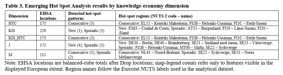
The temporal meaning of these categories sharpens the regional interpretation. HTC and KIS_HTC show only Consecutive Hot Spots (EL52, FI1B and FI1C), pointing to a recent multi-year run of concentrated high-intensity reweighting in the same regional systems. J has the broadest detected restructuring profile: DE30, DE40, SE21 and SE23 are New Hot Spots, suggesting a newly emerging 2025 concentration of intense restructuring, while FI1B, MT00 and SE22 are Sporadic Hot Spots, indicating recurrent but discontinuous adjustment. KIS combines one new trajectory (ES63) with sporadic adjustment in AT11, FI19 and FI20. M combines one consecutive trajectory (NL41) with sporadic patterns in SE31 and SE22. Most detected trajectories form a relatively compact northern-to north-western/central European core, especially across Finland, Sweden, Germany, the Netherlands, and Austria, with a small number of southern outliers.

 

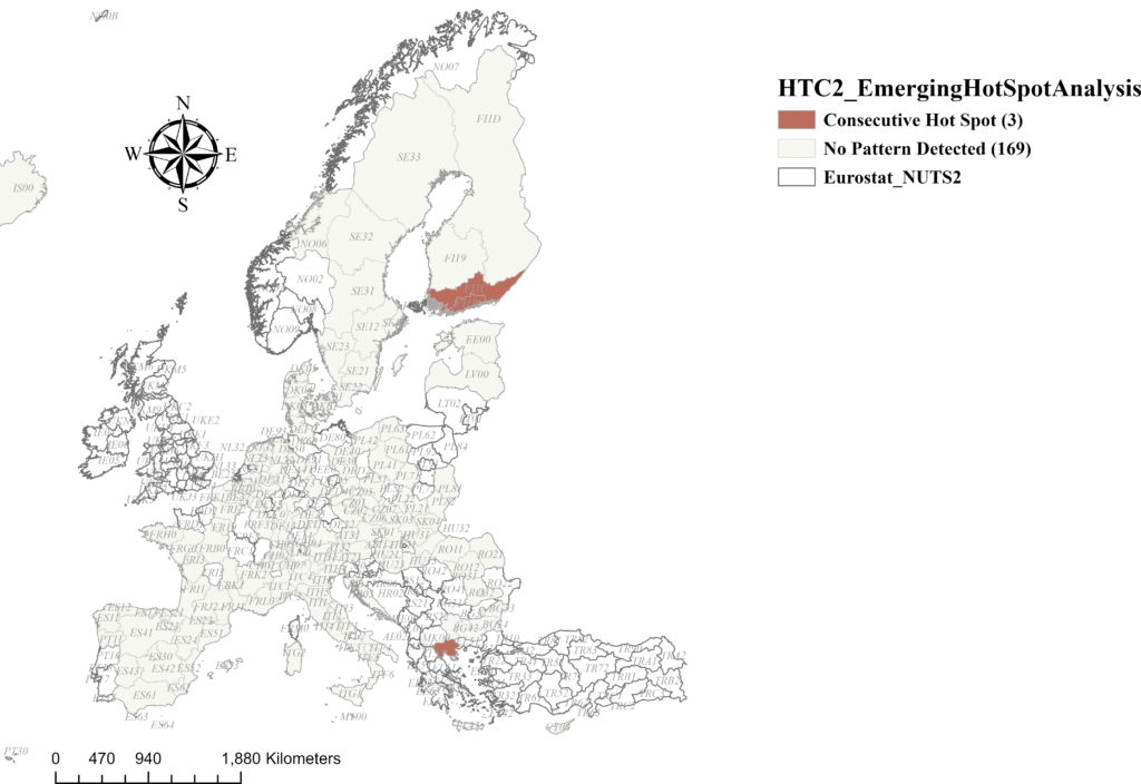
Figure 1. EHSA classification of SCI for HTC, 2009–2025.

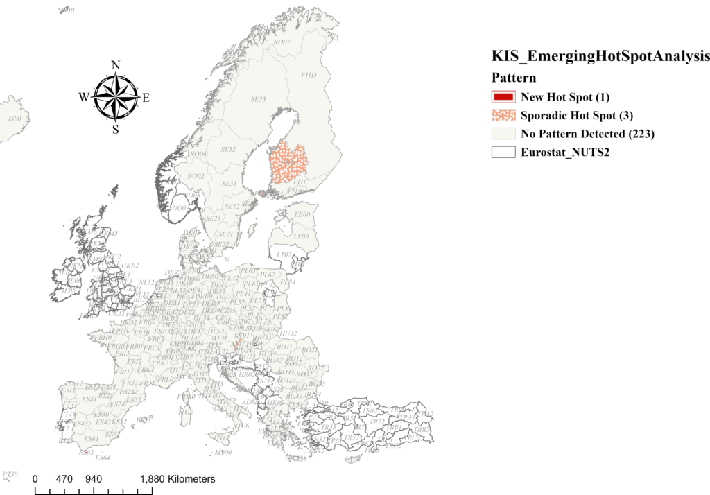
Figure 2. EHSA classification of SCI for KIS, 2009–2025.

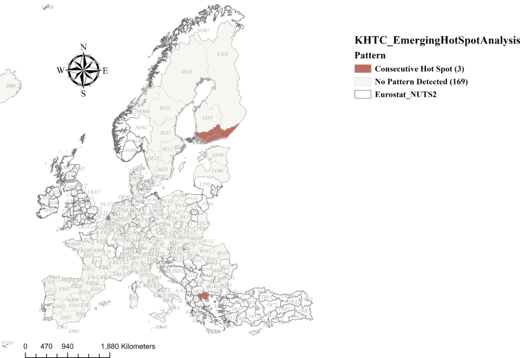
Figure 3. EHSA classification of SCI for KIS_HTC, 2009–2025.

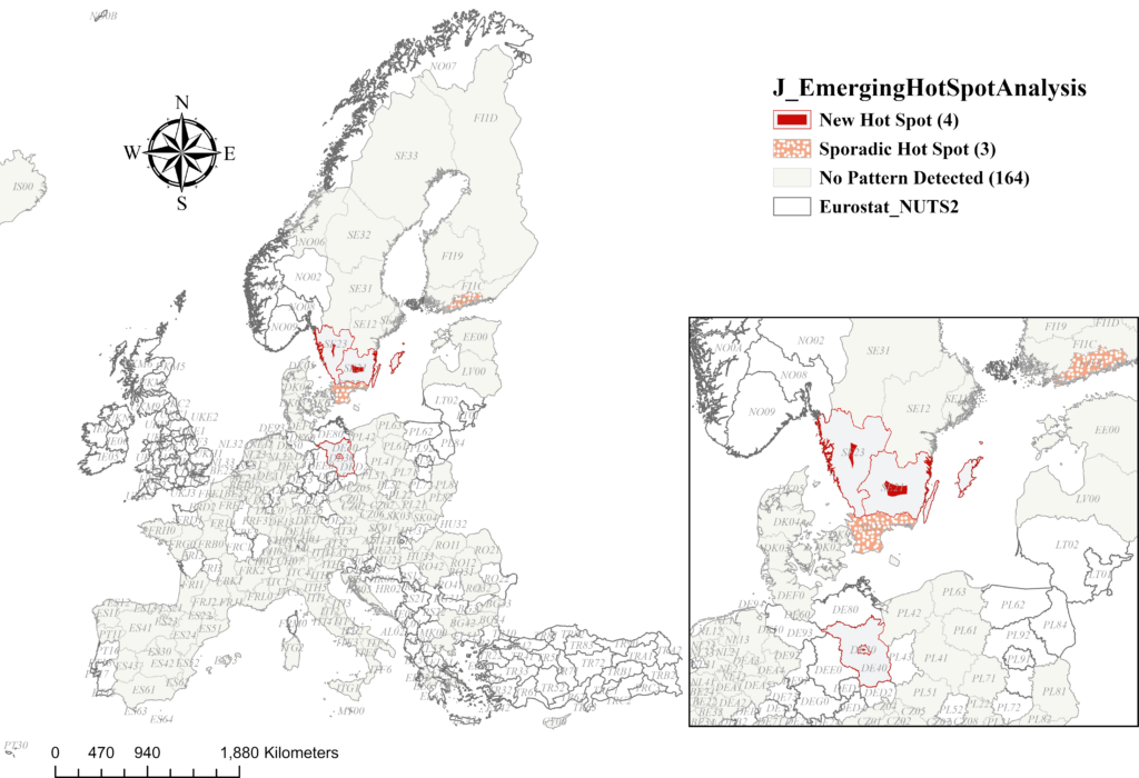
Figure 4. EHSA classification of SCI for J, 2009–2025.

 

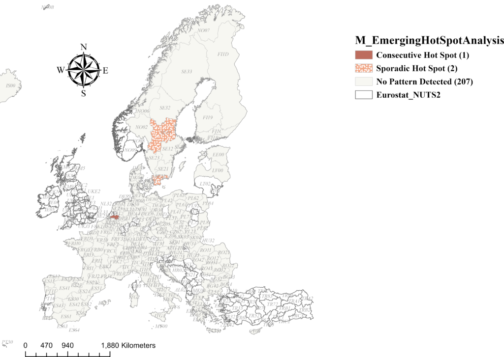
Figure 5. EHSA classification of SCI for M, 2009–2025.

Discussion and conclusions

Intersectoral reallocation matters because structural change must be absorbed through regional labour and skill systems. The three EHSA categories indicate different temporal regimes of adjustment. New hot spots mark the emergence of fresh restructuring pressure; consecutive hot spots indicate that this pressure has persisted across recent years; sporadic hot spots indicate repeated but discontinuous adjustment. None of these categories is intrinsically successful or unsuccessful adaptation: because SCI is direction-neutral, they identify the timing and persistence of reallocation pressure, while signed Δ and PC_EMP are needed to determine whether the underlying trajectory is expansion or contraction.

A remaining limitation is sample comparability: indicator-specific missingness and NUTS changes affect the balanced panels, while Drop locations deliberately trade spatial coverage for a non-imputed design.

Framed this way, intersectoral mobility and regional adaptation are directly connected at the aggregate regional level: changing sectoral employment shares provide the reallocation signal, while EHSA distinguishes newly emerging, sustained-recent and recurrent-episodic geographies of adjustment. Their concentration in a limited northern/north-western European core suggests that knowledge-economy restructuring—and the associated implications for skills adaptation—is place-specific rather than a uniform European process.

Acknowledgements

This contribution was developed within Project 5 (CAIS-TRANZDIVI) of the INCSMPS Nucleu Programme.

Declaration of generative AI use

OpenAI ChatGPT (GPT-5) was used for language refinement, bibliographic consistency checks and document formatting. The authors verified all content and take full responsibility for the final manuscript.

References

Boschma, R. (2015). Towards an evolutionary perspective on regional resilience. Regional Studies, 49(5), 733–751. https://doi.org/10.1080/00343404.2014.959481

Esri. (n.d.). How Emerging Hot Spot Analysis works. ArcGIS Pro documentation. Retrieved September 6, 2026, from https://pro.arcgis.com/en/pro-app/latest/tool-reference/space-time-pattern-mining/learnmoreemerging.htm

Eurostat. (2024). High-tech industry and knowledge-intensive services (htec) [Reference metadata]. https://ec.europa.eu/eurostat/cache/metadata/en/htec_esms.htm

Eurostat. (2026). Employed persons in technology and knowledge-intensive sectors by NACE Rev. 2 activity and NUTS 2 region (htec_emp_reg2) [Data set; data extracted 30 June 2026]. https://doi.org/10.2908/htec_emp_reg2

Getis, A., & Ord, J. K. (1992). The analysis of spatial association by use of distance statistics. Geographical Analysis, 24(3), 189–206. https://doi.org/10.1111/j.1538-4632.1992.tb00261.x

Herrendorf, B., Rogerson, R., & Valentinyi, Á. (2014). Growth and structural transformation. In P. Aghion & S. N. Durlauf (Eds.), Handbook of Economic Growth (Vol. 2, pp. 855–941). Elsevier. https://doi.org/10.1016/B978-0-444-53540-5.00006-9

OECD. (2026). OECD Employment Outlook 2026: Geographic Disparities in Jobs and Incomes. OECD Publishing. https://doi.org/10.1787/7e710f54-en

Ord, J. K., & Getis, A. (1995). Local spatial autocorrelation statistics: Distributional issues and an application. Geographical Analysis, 27(4), 286–306. https://doi.org/10.1111/j.1538-4632.1995.tb00912.x

Vu, K. M. (2017). Structural change and economic growth: Empirical evidence and policy insights from Asian economies. Structural Change and Economic Dynamics, 41, 64–77. https://doi.org/10.1016/j.strueco.2017.04.002